Create an Icon Map in R with ggmap and ggimage

Icon Maps with GGMap and GGImage in R

Previously I have written a tutorial on how to use ggmap with R. It provides the end to end instructions on how to get started with using ggmaps, including signing up for the google service and working with your API key.

This icon map tutorial is going to extend our ggmap work to create icon maps with ggmap and ggimage.

Set up packages

Uncomment any "install.packages()" lines if you also need to install the package.

#install.packages("tidyverse")
library(tidyverse)

#install.packages("readr")
library(readr)

#install.packages("proj4")
library(proj4)

#install.packages("magick")
library(magick)

#install.packages("ggmap")
library(ggmap)

#install.packages("ggimage")
library(ggimage)

Download the data

I was able to find some neat location information on the data portal for my home town, London Ontario.

In their catalogue, they have a variety of spreadsheets with location information of public facilities. I downloaded all public facilities of interest, combined and standardized them.

#Download the data set
df= read_csv('https://raw.githubusercontent.com/lgellis/MiscTutorial/master/iconmap/MasterList.csv', col_names = TRUE)

#Set your API Key  
#ggmap::register_google(key = "ENTER_YOUR_API_KEY")

*For more information about the API key, see my full ggmap tutorial.

Convert UTM to lat and long

In working with this dataset, I was very confused as to what the provided x and y coordinates were representing. After looking at their Q&A I realized that they are in Universal Transverse Mercator (UTM) format.

I found a way to convert UTM to Lat and Long from stack overflow. I slightly modified the code to run through the whole data set efficiently.

#Convert UTM to lat/lon

proj4string <- "+proj=utm +zone=17 +north +ellps=WGS84 +datum=NAD83 +units=m +no_defs "
nRow <- nrow(df)
df$Lat <-0
df$Lon <-0


for(i in 1:nRow){
  temp <-project(df[i,4:5], proj4string, inverse=TRUE)
  df[i,6] <- temp$y
  df[i,7] <-temp$x
}

Create the starting ggmap in R

I start out with a basic map plotting all amenities, colored by facility type. Again, for more information on the basics of ggmap, please see this tutorial.

p <- ggmap(get_googlemap(center = c(lon =-81.23304, lat = 42.98339),
                    zoom = 12, scale = 2,
                    maptype ='roadmap',
                    color = 'color'))

p + geom_point(aes(x = Lon, y = Lat,  colour = Facility), data = df, size = 0.5) + 
  theme(legend.position="bottom")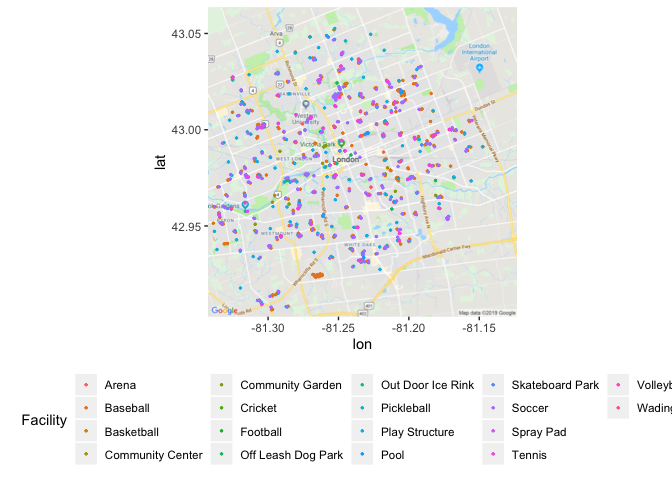

Filter and plot an icon map with GGImage in R

Filter to only include water facilities (pool, wading pool, spray pad).

Assign and display the icon for each facility type.

df2 <-df %>% 
  filter(Facility %in% c("Pool", "Wading Pool", "Spray Pad")) %>% 
  mutate(Image = case_when(Facility == "Pool" ~ "https://raw.githubusercontent.com/lgellis/MiscTutorial/master/iconmap/swimmer.png",
                           Facility == "Wading Pool" ~ "https://raw.githubusercontent.com/lgellis/MiscTutorial/master/iconmap/duckie.png", 
                           Facility == "Spray Pad" ~ "https://raw.githubusercontent.com/lgellis/MiscTutorial/master/iconmap/splash.png"))

p + geom_image(aes(x = Lon, y = Lat, image=Image), data = df2, size = 0.05) + 
  theme(legend.position="bottom")  

Prepare Images for ggimage

That was ok, but we should try to make the images more aesthetically pleasing using the magick package. We make each image transparent with the image_transparent() function. We can also make the resulting image a specific color with image_colorize().

I then saved the images using the image_write() function. I manually re-uploaded them to GH.

baby <-image_transparent(image_read("https://raw.githubusercontent.com/lgellis/MiscTutorial/master/iconmap/duckie.png"), 'white')
baby <- image_colorize(baby, 100, "#FF9933")
image_write(baby, path = "babyPoolFinal.png", format = "png")

swimmer <-image_transparent(image_read("https://raw.githubusercontent.com/lgellis/MiscTutorial/master/iconmap/swimmer.png"), 'white')
swimmer <- image_colorize(swimmer, 100, "#000099")
image_write(swimmer, path = "swimmerFinal.png", format = "png")

splash <-image_transparent(image_read("https://raw.githubusercontent.com/lgellis/MiscTutorial/master/iconmap/splash.png"), 'white')
splash <- image_colorize(splash, 100, "#3399FF")
image_write(splash, path = "splashFinal.png", format = "png")

Create a better map using the newly formatted icons

df2 <-df %>% 
  filter(Facility %in% c("Pool", "Wading Pool", "Spray Pad")) %>% 
  mutate(Image = case_when(Facility == "Pool" ~ "https://raw.githubusercontent.com/lgellis/MiscTutorial/master/iconmap/swimmerFinal.png",
                           Facility == "Wading Pool" ~ "https://raw.githubusercontent.com/lgellis/MiscTutorial/master/iconmap/babyPoolFinal.png", 
                           Facility == "Spray Pad" ~ "https://raw.githubusercontent.com/lgellis/MiscTutorial/master/iconmap/splashFinal.png"))

p + geom_image(aes(x = Lon, y = Lat, image=Image), data = df2, size = 0.06) + 
  theme(legend.position="bottom") 

Create a new version of the ggimage and ggmap viz using 'terrain-lines'

Now that we’ve sorted out our icons and have them plotted on the map, let’s try swapping out the base map. We are going to try the 'stamen' 'terrain-lines' version. I think that this a really cool way of looking at it as it represents the subdivisions more clearly.

For more information on swapping out base plots, please see my previous tutorial.

center = c(lon =-81.23304, lat = 42.98339)
qmap(center, zoom = 12, source = "stamen", maptype = "terrain-lines") +
  geom_image(aes(x = Lon, y = Lat, image=Image), data = df2, size = 0.06) + 
  theme(legend.position="bottom") 

Create a new version of the ggimage and ggmap viz using 'terrain'

Now swap out 'terrain-lines' for 'terrain'. I think this is my favorite version as it nicely balances showing green space and street lines very clearly at a distance.

center = c(lon =-81.23304, lat = 42.98339)
qmap(center, zoom = 12, source = "stamen", maptype = "terrain") +
  geom_image(aes(x = Lon, y = Lat, image=Image), data = df2, size = 0.06) + 
  theme(legend.position="bottom") 

Next Steps

If you liked this tutorial, you may be interested in a few other tutorials on this blog. Please check out:

Creating super easy U.S. maps with the usmaps package (no API key or shape files needed)

• Creating easy maps in R using ggmap

• Creating super easy U.S. maps with the usmaps package (no API key or shape files needed)
  
  

Thank You

Thank you for following along on this icon map tutorial with me.  Please comment below if you enjoyed this blog, have questions, or would like to see something different in the future.  Note that the full code is available on my  github repo.  

If you have trouble downloading the files or cloning the repo from github, please go to the main page of the repo and select "Clone or Download" and then "Download Zip". Alternatively or you can execute the following R commands to download the whole repo through R

install.packages("usethis")
library(usethis)
use_course("https://github.com/lgellis/MiscTutorial/archive/master.zip")